Definition
In probability theory and statistics, moments are a set of quantitative measures that describe the shape and characteristics of a probability distribution. They are derived from the powers of the random variable and they help in understanding properties like central tendency, dispersion, asymmetry, and peakedness of the distribution.
Why the Term "Moment"?
The term "moment" is borrowed from physics. In mechanics, the moment of inertia measures how mass is distributed relative to a reference point. Similarly, in probability theory, statistical moments describe how probability mass is distributed around a reference point like the mean.
In summary, mean and variance are called moments because they are special cases of the general concept of moments that describe different aspects of a probability distribution.
Types of Moments
Moments can be classified into two categories:
- Raw Moments (About the Origin): These are taken with respect to the origin (0).
- Central Moments (About the Mean): These are taken with respect to the mean of the distribution.
Raw Moments
The nth raw moment is defined as:
μn′ = E[Xn]
where:
- X is the random variable.
- n is the order of the moment.
- E[⋅] denotes the expectation operator.
Examples:
- First raw moment: μ1′ = E[X] (Mean of the distribution)
- Second raw moment: μ2′ = E[X2]
- Third raw moment: μ3′ = E[X3]
Central Moments
The nth central moment is defined as:
μn = E[ (X - μ)n]
where:
- X is the random variable.
- n is the order of the moment.
- E[⋅] denotes the expectation operator.
- μ = E[X] is the mean of the distribution
Examples:
- First central moment: μ1 = 0 (By definition, since the mean is subtracted)
- Second central moment: μ2 = E[(X−μ)2], which is the variance.
- Third central moment: μ3 = E[(X−μ)3], which measures skewness.
- Fourth central moment: μ4 = E[(X−μ)4], which measures kurtosis.
- Higher-Order Moments: 5th moment and beyond can capture more intricate details of the distribution, but they are less commonly used in practice.
Significance of Moments
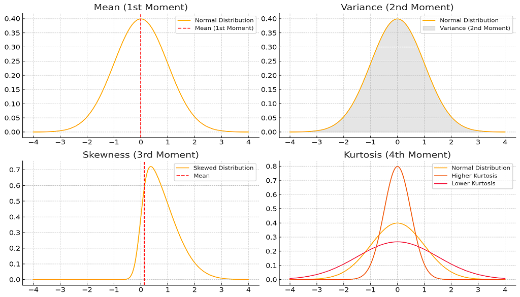
1. Mean (1st Moment - Center of Mass : E[X] )
Represents the central location of the distribution. It represents the "balance point" of the distribution. For symmetric distributions like the Normal Distribution, the mean is at the center.
When we have a set of data, the first thing we would like to know is where most of the data is located, that is, what is the central location of the data. For example, if we have set of marks between 0 and 100, scored by the students of a class in an exam, when we set out to analyse these marks, the very first thing we would want to know is what marks have mostly been scored by the students, that is, on the 0 to 100 scale where most of the marks lie. That is, we would want to know the "central location" of the marks data.
For example, in a particular exam, most of the marks scored by the students may be around 70.
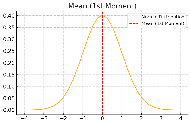
2. Variance (2nd Moment - Spread or Dispersion : E[(X−μ)2])
Measures the spread or dispersion around the mean. It measures how far the data points deviate from the mean. A higher variance indicates more spread-out data.
After knowing the central location of the data, the next thing we would want to know is how much spread apart are the data from the central location. This gives us insights that can help us is making decisions. For example, consider the following 4 cases:
1) The mean marks of the class is 80 and all the marks are between 60 and 100. This tells us that the class has all bright students,
2) The mean marks of the class is 80 and all the marks are between 15 and 100. This tells us that the class has mostly bright students but there are some very dull students,
3) The mean marks of the class is 50 and all the marks are between 10 and 100. This tells us that the class has mostly ordinary students but there are some very bright students and some very dull students,
4) The mean marks of the class is 50 and all the marks are between 40 and 60. This tells us that the class has all very ordinary students, none too bright and none too dull.
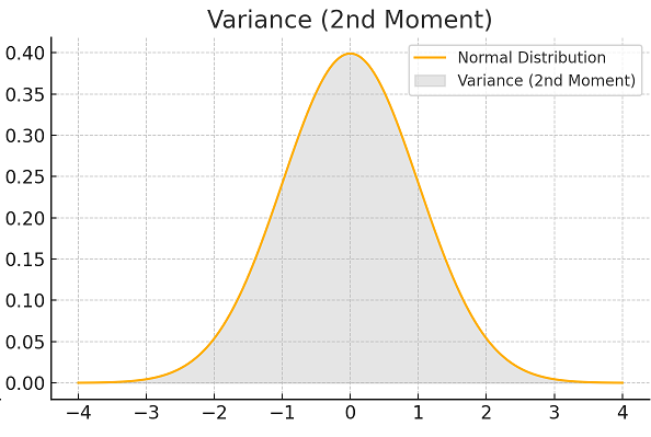
3. Skewness (3rd Moment - Asymmetry : E[(X−μ)3] )
Measures the asymmetry of the distribution.
- Positive skew: Right tail is longer.
- Negative skew: Left tail is longer.
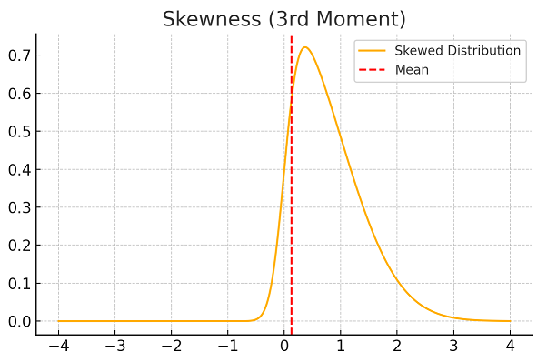
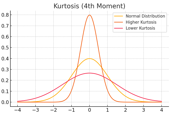
4. Kurtosis (4th Moment : E[(X−μ)4])
Measures the "fatness" or "thinness" of the tails or the concentration of values around the mean. Fatness and thinness are relative words, one can be called fat or thin only in comparision to something else, In this case, the relative fatness or thinness is measured in comparison to a "Normal" distribution.
- High kurtosis (Leptokurtosis): Heavy tails (outliers). Most of the data lies either around the mean or in the tails, much less data lie at a medium distance from the mean when compared to a "Normal" distribution.
- Low kurtosis (Platykurtosis): Light tails. Much less data lies around the mean and in the tails whereas much more data lie at a medium distance from the mean when compared to a "Normal" distribution
- Medium kurtosis (Mesokurtosis): Average tails. as much data lies around the mean, in the tails and at a medium distance from the mean as in a "Normal" distribution
Standardized Moments
To make moments dimensionless and easier to compare across distributions, standardized moments are used. They are defined as:
μ~n = μn / σn
where σ is the standard deviation.
- Standardized Skewness: μ3 = E[(X−μ)3] / σ3
- Standardized Kurtosis: μ4 = E[(X−μ)4] / σ4
Applications of Moments
- Descriptive Statistics: Understanding the shape of the distribution (mean, variance, skewness, kurtosis).
- Statistical Inference: Estimating population parameters.
- Machine Learning: Feature engineering and data transformation.
- Financial Analytics: Analyzing returns and risk.